
The question
After ten years of gravitating around Las Palmas (see my stops here), I decided it was time to buy a house. But where? In ten years, prices had risen fast in the most popular areas, with no sign of slowing down. And for me it wasn’t just a place to stay: I wanted to keep travelling from time to time, so it also had to be a good investment, and possibly a great deal!
So, how do you find a great deal? My studies in Python and data came in handy, and early AI (it was late 2023) helped me with some of the code and some financial concepts. One of them was the PRR, or price-to-rent ratio, which isn’t exactly something you pick up at school or in most walks of life. In other words: in which areas are sale prices lowest compared to rents? That’s what my Jupyter notebook set out to answer, using several downloads of listings from Idealista, a popular property website in Spain, Italy and Portugal.
The data
I pulled the listings through an Idealista API available on RapidAPI. A script downloads every page of listings, both for sale and for rent, and saves them as JSON files. Older downloads are archived with their date, so nothing gets overwritten.
Then the cleaning:
- Price per m²: each listing’s price divided by its size, which makes small flats and big houses comparable.
- Duplicates: removed, since the same listing can appear on more than one page.
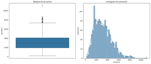
- Outliers: I checked the distribution with a boxplot and a histogram, then kept sales and rents within reasonable limits, cutting off a few extreme listings (above €9,000 per m², for example).
- City limits: only listings inside a box drawn around Las Palmas.
The map
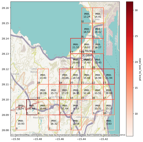
I split the city into a grid and tried several sizes (10×10, 20×20…). Smaller cells show more detail, but each one holds fewer listings, so the averages get less reliable. For each cell, the notebook takes the average price per m² of the homes for sale and of the homes for rent, and keeps only the cells that have both.
Then the key number: the price-to-rent ratio, which is the sale price per m² divided by a year’s rent per m². Put simply, it’s roughly how many years of rent it takes to pay back the purchase price, before taxes and other costs like renovation, furniture and maintenance. In any case, the lower the ratio, the more convenient it is to buy there.
Finally, the grid is drawn over a map of Las Palmas (OpenStreetMap). Each cell shows its ratio, and the outline gets a darker red as the ratio rises. At a glance, the pale cells are where to start looking.
From map to house
The map didn’t pick the house. It told me where to look. I took the most promising cells and zoomed in:
- The listings: a second map plotted every listing as a clickable marker, with price, size and price per m², linking straight to the ad.
- The area itself: then I went and checked the neighbourhoods in person.
- The deal: the rest was negotiating with the owner, something we’re still better off not automating. 🙂
That’s how I found the house I bought in spring 2024.
Limits
It’s a compass, not a valuation:
- Asking prices: listings show what owners hope to get, not what homes actually sell or rent for.
- Thin cells: a cell with only a few listings gives an average that one odd listing can swing.
- A snapshot: the data reflects the day it was downloaded, and the market keeps moving.
- Not the whole cost: the ratio leaves out taxes, renovation, furniture, maintenance and empty months between tenants.
- Mixed listings: from brand-new homes to ones that need a full renovation, they all count the same in the average. Some listings are auctions, and some come with unusual deals (for example, you buy the home, but the current occupant keeps the right to live in it). Others come with conditions that a simple script can’t read.
Today, an AI could read every ad and flag those cases. I didn’t have that at the time, but there were few enough listings that I could check them myself.